isotopylog.kDistribution

class isotopylog.kDistribution(params, model, T, **kwargs)

Class for inputting, storing, and visualizing clumped isotope rate data. Currently only accepts D47 clumps, but will be expanded in the future as new clumped system data becomes available.

Parameters:

• params (array-like) –

  A list of the rate parameters associated with a given kDistribution. The values and length of this array depend on the type of model being implemented:

  'Hea14': [ln(kc), ln(kd), ln(k2)]

  'HH21': [ln(k_mu), ln(k_sig)]

  'PH12': [ln(k), intercept]

  'SE15': [ln(k1), ln(k_dif_single), ln([pair]_0/[pair]_eq)]

  See discussion in each reference for parameter definitions and further details. All k values should be in units of inverse time, although the exact time unit can change depending on inputs.

• model (string) – The type of model associated with a given kDistribution. Options are: 'Hea14', 'HH21', 'PH12', or 'SE15'.
• nu (None or array-like) – The ln(k) values over which the rate distribution is calculated. nu only applies when model = 'HH21'. Defaults to None.
• npt (None or int) – The number of data points used in the model fit. If model = 'Hea14' or model = 'PH12', then npt is the number of points deemed to be in the linear region of the curve; otherwise, it is all data points. Defaults to None.
• omega (None or scalar) – The Tikhonov omega value used for inverse regularization. omega only applies when model = 'HH21' and fit_reg = True. Defaults to None.
• params_cov (None or array-like) – Covariance matrix of the parameters, of shape [nparams``x``nparams]. The +/- 1 sigma uncertainty for each parameter is calculated as np.sqrt(np.diag(params_cov)). Defaults to None.
• rho_nu (None or array-like) – The modeled lognormal probability density function of ln(k) values. rho_nu only applies when model = 'HH21'. Defaults to None.
• rho_nu_inv (None or array-like) – The modeled inverse probability density function of ln(k) values calculated using Tikhonov regularization. rho_nu_inv only applies when model = 'HH21' and fit_reg = True. Defaults to None.
• res_inv (None or float) – The residual norm the Tikhonov regularization model-data fit, in D47 units. res_inv only applies when model = 'HH21' and fit_reg = True. Defaults to None.
• rgh_inv (None or float) – The roughness norm the Tikhonov regularization model-data fit. res_inv only applies when model = 'HH21' and fit_reg = True. Defaults to None.
• rmse (None or float) – The root-mean-square-error of the model-data fit, in D47 units. Defaults to None.

Raises:

• TypeError – If inputted parameters of an unacceptable type.
• ValueError – If an unexpected keyword argument is trying to be inputted.
• ValueError – If an unexpected model name is trying to be inputted.

See also

isotopylog.EDistribution

The class for combining multiple kDistribution instances and determining the underlying activation energies.

isotopylog.HeatingExperiment

The class containing heating experiment clumped isotope data whose rate data are determined.

Examples

Generating a bare-bones kDistribution instance without fitting any actual data:

#import packages
import isotopylog as ipl

#assume some values for HH21 model parameters
params = [-14., 5.]

#make instance
kd = ipl.kDistribution(params, 'HH21')

Assuming some EDistribution instance exists, rate data can be calculated simply as:

#import packages
import isotopylog as ipl

#say, calculate data at 425 C
T = 425 + 273.15

#assuming EDistribution instance, ed
kd = ipl.kDistribution.from_EDistribution(ed, T)

Alternatively, one can generate a kDistribution instance by fitting some experimental D47 data contained in a HeatingExperiment object:

#assume some he is a HeatingExperiment object
kd = ipl.kDistribution.invert_experiment(he, model = 'PH12')

Same as above, but now including the Tikhonov regularization inverse fit for ‘HH21’ model type:

#assume some he is a HeatingExperiment object
kd = ipl.kDistribution.invert_experiment(
        he,
        model = 'HH21',
        fit_reg = True
        )

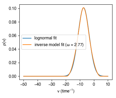
To visualize these results, we can generate a plot of ‘HH21’ model k distributions:

#import necessary packages
import matplotlib.pyplot as plt

#make axis
fig, ax = plt.subplots(1,1)

#plot data
kd.plot(ax = ax)

Export summary information for storing and saving:

sum_tab = kd.summary
sum_tab.to_csv('file_name.csv')

References

[1] Hansen (1994) Numerical Algorithms, 6, 1-35.

[2] Forney and Rothman (2012) J. Royal Soc. Inter., 9, 2255–2267.

[3] Passey and Henkes (2012) Earth Planet. Sci. Lett., 351, 223–236.

[4] Henkes et al. (2014) Geochim. Cosmochim. Ac., 139, 362–382.

[5] Stolper and Eiler (2015) Am. J. Sci., 315, 363–411.

[6] Daëron et al. (2016) Chem. Geol., 442, 83–96.

[7] Hemingway and Henkes (2021) Earth Planet. Sci. Lett., 566, 116962.

__init__(params, model, T, **kwargs)

Initilizes the object.

Returns:kd – The kDistribution object. Return type:isotopylog.kDistribution

Methods

__init__(params, model, T, **kwargs)	Initilizes the object.
from_EDistribution(ed, T)	Classmethod for generating rate data directly from activation energy data.
invert_experiment(he[, model, fit_reg])	Classmethod for generating a kDistribution instance directly by inverting a ipl.HeatingExperiment object that contains clumped isotope heating experiment data.
plot([ax, lnd, invd])	Generates a plot of ln(k) distributions for ‘HH21’-type models.

Attributes

T	The temperature for which the rate data correspond, in Kelivn.
model	The type of model associated with a given kDistribution.
npt	The number of data points used in the model fit.
nu	The ln(k) values over which the rate distribution is calculated.
omega	The Tikhonov omega value used for inverse regularization.
params	A list of the rate parameters associated with a given kDistribution.
params_cov	Uncertainty associated with each parameter value, as +/- 1 sigma.
res_inv	The residual norm the Tikhonov regularization model-data fit.
rgh_inv	The roughness norm the Tikhonov regularization model-data fit.
rho_nu	The modeled lognormal probability density function of ln(k) values.
rho_nu_inv	The modeled inverse probability density function of ln(k) values calculated using Tikhonov regularization.
rmse	The root-mean-square-error of the model-data fit.
summary	Series containing all the summary data.