isotopylog.EDistribution.plot
-
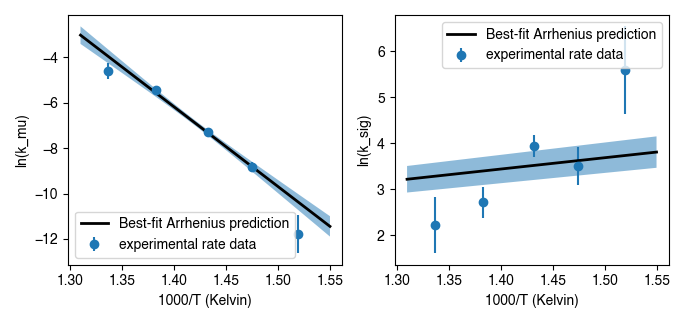
EDistribution.plot(ax=None, nT=300, param=1, eps=1e-06, ed={'fmt': 'o'}, ld={}, fbd={'alpha': 0.5})¶ Generates an Arrhenius plot of a given parameter.
Parameters: - ax (None or plt.axis) – Axis for plotting results; defaults to None.
- nT (int) – The number of temperature points to plot for Arrhenius fit predictions.
- param (int) –
The parameter of interest for making Arrhenius plot, specific to each model as follows:
'Hea14': [ln(kc), ln(kd), ln(k2)]'HH21': [ln(k_mu), ln(k_sig)]'PH12': [ln(k), intercept]'SE15': [ln(k1), ln(k_dif_single), ln([pair]_0/[pair]_eq)]For eample, to make an Arrhenius plot of ln(kc) for ‘Hea14’ models, pass
param = 1. - eps (float) – The amount to perturb each parameter when numerically calculating
the derivative of ln(k) with respect to each parameter. Used for
calculating a Jacobian to propagate parameter uncertainty. Defaults
to
1e-6. - ed (dictionary) – Dictionary of keyward arguments to pass for plotting the
experimental data. Must contain keywords compatible with
matplotlib.pyplot.errorbar. Defaults to dictionary with ‘fmt’ = ‘o’. - ld (dictionary) – Dictionary of keyward arguments to pass for plotting the mean of
the Arrhenius model fit line. Must contain keywords compatible with
matplotlib.pyplot.plot. Defaults to empty dictionary. - fbd (dictionary) –
Dictionary of keyward arguments to pass for plotting the Arrhenius model uncertaint range. Must contain keywords compatible with
matplotlib.pyplot.errorbar. Defaults to dictionary with ‘alpha’= 0.5..
Returns: ax – Updated axis containing results.
Return type: plt.axis
Raises: ValueError– If passedparamis outside of the range of existing parameters (e.g., >2 for ‘HH21’ models).See also
isotopylog.kDistribution.plot()- Class method for plotting rate distributions for ‘HH21’ model types.
Examples
Basic implementation, assuming
ipl.EDistributioninstanceedexists and contains data of model type ‘HH21’:#import modules import isotopylog as ipl import matplotlib.pyplot as plt #make figure fig, ax = plt.subplots(2, 1, sharex = True) #plot results ed.plot(ax = ax[0], param = 1) #to plot mu_E ed.plot(ax = ax[1], param = 2) #to plot sig_E
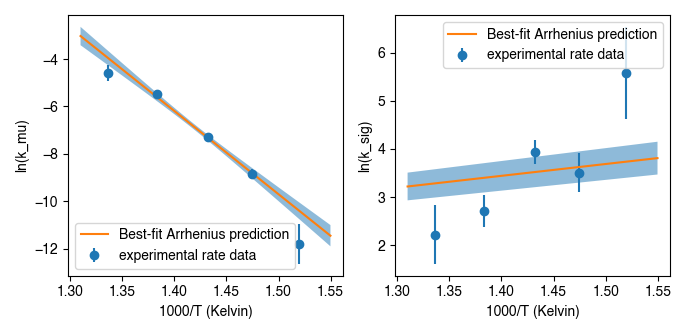
Similar implementation, but now putting in stylistic keyword args:
#import modules
import isotopylog as ipl
import matplotlib.pyplot as plt

#make figure
fig, ax = plt.subplots(2, 1, sharex = True)

#define plotting style
ld = {'linewidth':2, 'c':'k'}

#plot results
ed.plot(ax = ax[0], param = 1, ld = ld) #to plot mu_E
ed.plot(ax = ax[1], param = 2, ld = ld) #to plot sig_E