isotopylog.calc_L_curve
-
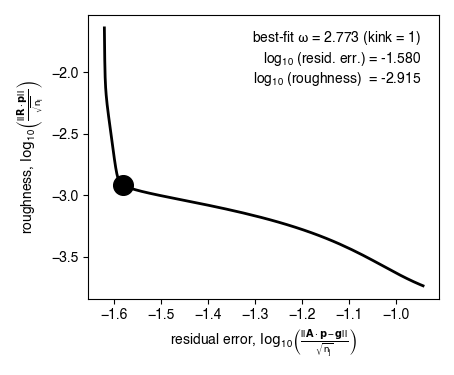
isotopylog.calc_L_curve(he, ax=None, kink=1, nu_max=10, nu_min=-50, nnu=300, nom=150, omega_max=100.0, omega_min=0.01, plot=False, ld={}, pd={})¶ Function to choose the “best” omega value for regularization following the Tikhonov Regularization method. The best-fit omega is chosen as the value at the point of maximum curvature in a plot of log residual error vs. log roughness.
Parameters: - he (isotopylog.HeatingExperiment) –
ipl.HeatingExperimentinstance containing the D data to be modeled. - ax (Non` or plt.axis) – Matplotlib axis to plot on, only relevant if
plot = True. - kink (int) – Tells the funciton which L-curve “kink” to use; this is a required input since some L-curve solutions appear to have 2 “kinks”; input 1 for the highest curvature kink and 2 for the second-highest curvature kink.
- nu_max (scalar) – Maximum nu value for distribution range; should be at least 4 sigma above the mean; defaults to 30.
- nu_min (scalar) – Minimum nu value for distribution range; should be at least 4 sigma below the mean; defaults to -30.
- nnu (int) – Number of nodes in nu array.
- nom (int) – Number of nodes on omega array.
- omega_max (float) – Maximum omega value to consider, defaults to 1e3.
- omega_min (float) – Minimum omega value to consider, defaults to 1e-3.
- plot (Boolean) – Boolean telling the funciton whether or not to plot L-curve results.
- ld (dictionary) – Dictionary of keyward arguments to pass for plotting the L-curve line.
Must contain keywords compatible with
matplotlib.pyplot.plot. Defaults to empty dictionary. Only called ifplot = True. - pd (dictionary) – Dictionary of keyward arguments to pass for plotting the best-fit omega
point. Must contain keywords compatible with
matplotlib.pyplot.scatter. Defaults to empty dictionary. Only called ifplot = True.
Returns: - om_best (float) – The ‘best fit’ omega value.
- ax (plt.axis or None) – Updated Matplotlib axis containing L-curve plot.
See also
isotopylog.fit_HH21inv()- Method for fitting heating experiment data using the L-curve approach of Hemingway and Henkes (2021).
kDistribution.invert_experiment()- Method for generating a kDistribution instance from experimental data; can generate L curve if model = “HH21” and fit_reg = True.
Examples
Basic implementation, assuming a ipl.HeatingExperiment instance he exists:
#import modules
import isotopylog as ipl

#assume he is a HeatingExperiment instance
om_best = ipl.calc_L_curve(he, plot = False)
Similar implementation, but now also generating a plot of the resulting L-curve:
#import modules
import matplotlib.pyplot as plt

#make axis instance
fig,ax = plt.subplots(1,1)

#pre-set stylistic arguments
ld = {'linewidth' : 2, 'color' : 'k'}
pd = {'s' : 200, 'color' : 'k'}

#assume he is a HeatingExperiment instance
om_best, ax = ipl.calc_L_curve(
        he,
        ax = ax,
        plot = True,
        ld = ld,
        pd = pd
        )
References
[1] Hansen (1994) Numerical Algorithms, 6, 1-35.
[2] Forney and Rothman (2012) J. Royal Soc. Inter., 9, 2255–2267.
[3] Hemingway and Henkes (2021) Earth Planet. Sci. Lett., X, XX–XX.
- he (isotopylog.HeatingExperiment) –