isotopylog.geologic_history
-
isotopylog.geologic_history(t, T, ed, d0, d0_std=[0.0, 0.0, 0.0], calibration='Aea21', iso_params='Brand', ref_frame='I-CDES', nnu=400, z=6, **kwargs)¶ Predicts the D47 evolution when a given
ipl.EDistributionmodel is subjected to any arbitrary time-temperature history.Parameters: - t (array-like) – Array of time points, in the same temporal units used to calculate
the
isotopylog.EDistributionobject passed to this function. Of lengthnt. - T (array-like) – Array of temperatures at each time point, in Kelvin. Of length
nt. - ed (isotopylog.EDistribution) – The
ipl.EDistributionobject containing the activation energy parameters used for forward modeling. - d0 (array-like) – Array of initial isotope composition, in the order [D47, d13C, d18O],
with d13C and d18O both reported relative to VPDB. Note that d13C and
d18O are only used if
ed.model = 'SE15'; for other model types, these are unused and arbitrary values can be passed. - d0_std (array-like) – Uncertainty associated with the values in d0, as +/- 1 standard deviation. Defaults to array of zeros.
- calibration (string or lambda function) –
The D-T calibration curve to use, either from the literature or as a user-inputted lambda function. If from the literature for D47 clumps, options are:
'PH12': for Passey and Henkes (2012) Eq. 4 (CDES 25C)'SE15': for Stolper and Eiler (2015) Fig. 3 (Ghosh 25C)'Bea17': for Bonifacie et al. (2017) Eq. 2 (CDES 90C)'Aea21': for Anderson et al. (2021) Eq. 1 (I-CDES)If as a lambda function, must have T in Kelvin. It is recommended to run each calibration only using its native reference frame (denoted in parentheses); although these will be automatically adjusted to different reference frames, there is no guarantee that this conversion is accurate for all analytical setups. In contrast, lambda functions must be reference-frame specific. Defaults to
'Aea21'. - iso_params (string) –
The isotope parameters used to calculate clumped data. For example, if
clumps = 'CO47', then isotope parameters are R13_vpdb, R17_vpdb, R18_vpdb, and lam17. Following Daëron et al. (2016) nomenclature, options are:'Barkan': for Barkan and Luz (2005) lam17'Brand'(equivalent to'Chang+Assonov'): for Brand (2010)'Chang+Li': for Chang and Li (1990) + Li et al. (1988)'Craig+Assonov': for Craig (1957) + Assonov and Brenninkmeijer (2003)'Craig+Li': for Craig (1957) + Li et al. (1988)'Gonfiantini': for Gonfiantini et al. (1995)'Passey': for Passey et al. (2014) lam17Defaults to
'Brand'. Only used ifed.model = 'SE15'. - ref_frame (str) –
The reference frame used to calculate clumped isotope data. Options are:
'CDES25': Carbion Dioxide Equilibrium Scale acidified at 25 C.'CDES90': Carbon Dioxide Equilibrium Scale acidified at 90 C.'Ghosh': Heated Gas Line Reference Frame of Ghosh et al. (2006) acidified at 25 C.'I-CDES': Carbon Dioxide Equilibrium Scale acidified at 90 C, referenced to carbonate standards as described in Bernasconi et al. (2021).Defaults to
'I-CDES'. - nnu (int) – The number of points to use in the nu array. Only applies if
ed.model = 'HH21'; for other model types, this is unused. Defaults to400. - z (int) – The mineral coordination number. Only applies if
ed.model = 'SE15'; for other model types, this is unused. Defaults to6as suggested in Stolper and Eiler (2015).
Returns: - D (np.array) – Array of resulting D47 values. Of length
nt. - D_std (np.array) – Array of corresponding uncertainty for resulting D values. Of length
nt.
Raises: TypeError– If inputted ‘calibration’ and/or ‘ref_frame’ are not strings or (lambda function).ValueError– If inputted t and T arrays are not the same length.ValueError– If inputted ‘calibration’ and/or ‘ref_frame’ arrays are not acceptable strings.
See also
isotopylog.EDistribution()- The class that contains the activation energy parameters that are to be modeled.
Examples
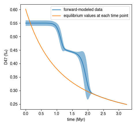
Estimate resetting temperatures during heating for an arbitrarily chosen starting isotope composition. This example creates an
ipl.EDistributioninstance by importing literature values of the ‘SE15’ model type, and plots results:#import packages import isotopylog as ipl import matplotlib.pyplot as plt #generate EDistribution instance ed = ipl.EDistribution.from_literature( mineral = 'calcite', reference = 'SE15', Tref = 700) #define the initial composition and the time-temperature evolutions d0 = [0.55, 0, 0] #starting D47 = 0.55, d13C and d18O both zero d0_std = [0.010, 0, 0] #assume some reasonable D47 uncertainty T0 = 25 + 273.15 #assume starting at 25C, ending at 350C Tf = 350 + 273.15 beta = 100/(1e6*365*24*3600) #100C/million years, converted to seconds t0 = 0 tf = (Tf-T0)/beta nt = 500 T = np.linspace(T0, Tf, nt) t = np.linspace(t0, tf, nt) #now calculate D at each time point D, Dstd = ipl.geologic_history(t, T, ed, d0, d0_std = d0_std) #plot results, along with equilibrium D at each time point Deq = ipl.Deq_from_T(T) tmyr = t/(1e6*365*24*3600) #getting t in Myr for plotting fig,ax = plt.subplots(1,1) ax.plot(tmyr, D, label = 'forward-modeled data') ax.fill_between(tmyr, D - Dstd, D + Dstd, alpha = 0.5) ax.plot(tmyr,Deq, label = 'equilibrium values at each time point') ax.set_xlabel('time (Myr)') ax.set_ylabel('D47 (‰)') ax.legend(loc = 'best')
Note the non-monotonic behavior that arises from the intermediate “pair” reservoir (see Stolper and Eiler 2015, Lloyd et al. 2018, and Chen et al., 2019 for further details).
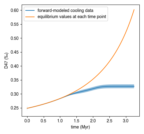
Similarly, one can estimate cooling closure temperatures. This is identical to the above example, only the temperature axis is reversed and D is assumed to be in equilibrium at T0:
#reverse T and Deq arrays
T = T[::-1]
Deq = Deq[::-1]

#make D0 in equilibrium
D0 = ipl.Deq_from_T(T[0])
d0 = [D0, 0, 0] #still d13C and d18O of zero

#fit the new t-T trajectory
D, Dstd = ipl.geologic_history(t, T, ed, d0, d0_std = d0_std)

#plot the results
fig,ax = plt.subplots(1,1)
ax.plot(tmyr, D, label = 'forward-modeled cooling data')
ax.fill_between(tmyr, D - Dstd, D + Dstd, alpha = 0.5)
ax.plot(tmyr,Deq, label = 'equilibrium values at each time point')

ax.set_xlabel('time (Myr)')
ax.set_ylabel('D47 (‰)')
ax.legend(loc = 'best')
References
[1] Passey and Henkes (2012) Earth Planet. Sci. Lett., 351, 223–236.
[2] Henkes et al. (2014) Geochim. Cosmochim. Ac., 139, 362–382.
[3] Stolper and Eiler (2015) Am. J. Sci., 315, 363–411.
[4] Lloyd et al. (2018) Geochim. Cosmochim. Ac., 242, 1–20.
[5] Chen et al. (2019) Geochim. Cosmochim. Ac., 258, 156–173.
[7] Hemingway and Henkes (2021) Earth Planet. Sci. Lett., 566, 116962.
- t (array-like) – Array of time points, in the same temporal units used to calculate
the