isotopylog.EDistribution

class isotopylog.EDistribution(kds, **kwargs)

Class for inputting, storing, and visualizing clumped isotope activation energies. Currently only accepts D47 clumps, but will be expanded in the future as new clumped system data becomes available.

Parameters:

• kds (list) – List of isotopylog.kDistribution objects over which to calculate activation energies.
• p0 (list) – List of initial guesses for fitting E parameters. Defaults to [150, -7], which should be adequate for all model fits.
• Tref (int) – The temperature at which the reference k value is calculated. Following Passey and Henkes (2012), this can be inputted directly in order to avoid large extrapolations in 1/T space. Defaults to np.inf; that is, defaults to k_ref = k0, the canonical Arrhenius pre-exponential factor.

Raises:

• TypeError – If attempting to pass kds that is not an iterable list of isotopylog.kDistribution and/or isotopylog.EDistribution objects.
• ValueError – If attempting to create an EDistribution object using kDistributions of multiple different model types.

Notes

All resulting activation energies are reported in units of kJ/mol. All resulting ln(kref) values are reported in units of ln inverse time, with one exception: ‘mp’, which is reported in units of Kelvin. This means that for ‘SE15’ E([pair]0/[pair]rand) should be zero and ln(kref)([pair]0/[pair]rand) should be equal to the slope mp analogous to that reported in Stolper and Eiler (2015) Eq. 17. IF E([pair]0/[pair]rand) IS NOT ZERO (or within a numerical rounding error of zero), THIS IMPLIES THAT ln([pair]0/[pair]rand) DEPENDS ON 1/T**2, NOT 1/T AS ASSUMED IN STOLPER AND EILER 2015.

For ‘HH21’ models, sig_nu is forced to an intercept of zero in 1/T vs. sig_nu space as discussed in Hemingway and Henkes (2021).

See also

isotopylog.kDistribution

The class containing rate data for individual experiments that is to be fit using Arrhenius plots.

Examples

Generating an EDistribution object from an existing list of kDistribution objects:

#import packages
import isotopylog as ipl

#assuming some list, kd_list, contains kDistributions at different T
ed = ipl.EDistribution(kd_list)

Alternatively, EDistribution objects can be generated directly from literature values:

#make EDistribution object
ed = ipl.EDistribution.from_literature(
        mineral = 'calcite',
        reference = 'PH12'
        )

If an EDistribution object exists, additional data points can also be appended to it. For example, adding an existing k distribution, kd, to an existing E distribution, ed:

ed.append(kd)

Alternatively, adding an existing E distribution, ed2, to a different E distribution, ed1, of the same model type:

ed1.append(ed2)

Similarly, individual data points can be dropped from an EDistribution object:

#say, drop element zero
ed.drop(0)

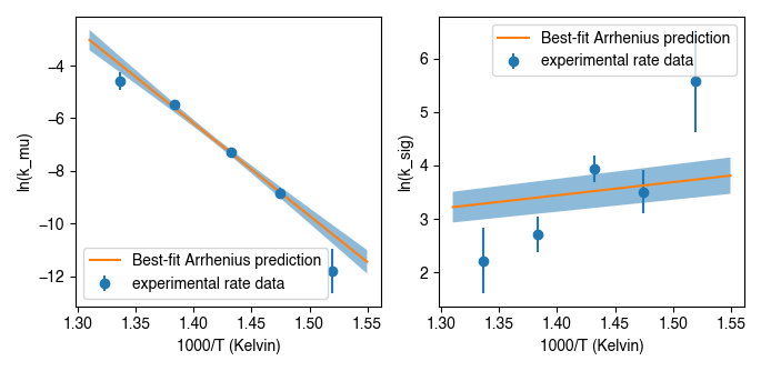
Finally, data can be visualized using Arrhenius plots. For example, assuming ipl.EDistribution instance ed exists and contains data of model type ‘HH21’:

#import additional packages
import matplotlib.pyplot as plt

#make figure
fig, ax = plt.subplots(1,2, sharex = True)

#plot results
ed.plot(ax = ax[0], param = 1) #to plot mu_E
ed.plot(ax = ax[1], param = 2) #to plot sig_E

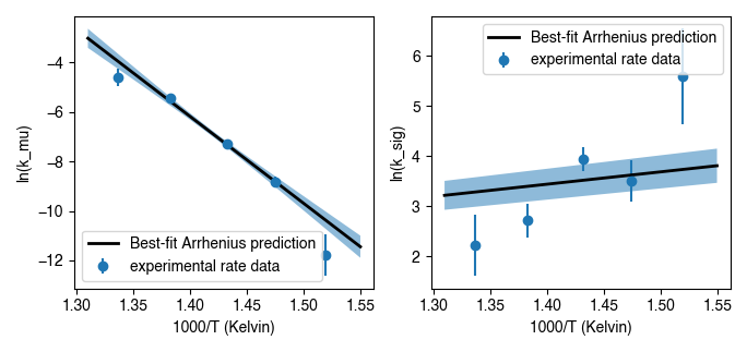
Similar implementation, but now putting in stylistic keyword args:

#import modules
import isotopylog as ipl
import matplotlib.pyplot as plt

#make figure
fig, ax = plt.subplots(1,2, sharex = True)

#define plotting style
ld = {'linewidth':2, 'c':'k'}

#plot results
ed.plot(ax = ax[0], param = 1, ld = ld) #to plot mu_E
ed.plot(ax = ax[1], param = 2, ld = ld) #to plot sig_E

References

[1] Passey and Henkes (2012) Earth Planet. Sci. Lett., 351, 223–236.

[2] Henkes et al. (2014) Geochim. Cosmochim. Ac., 139, 362–382.

[3] Stolper and Eiler (2015) Am. J. Sci., 315, 363–411.

[4] Brenner et al. (2018) Geochim. Cosmochim. Ac., 224, 42–63.

[5] Lloyd et al. (2018) Geochim. Cosmochim. Ac., 242, 1–20.

[6] Hemingway and Henkes (2021) Earth Planet. Sci. Lett., 566, 116962.

[7] Looser et al. (2023) Geochim. Cosmochim. Ac., 350, 1–15.

__init__(kds, **kwargs)

Initilizes the object.

Returns:ed – The EDistribution object. Return type:isotopylog.kDistribution

Methods

__init__(kds, **kwargs)	Initilizes the object.
append(new_data)	Method for appending new data onto an existing EDistribution.
drop(index)	Method for dropping entries from the existing list of k values.
from_literature([mineral, reference])	Classmethod for generating an ipl.EDistribution instance directly from literature data.
plot([ax, nT, param, eps, ed, ld, fbd])	Generates an Arrhenius plot of a given parameter.

Attributes

Eparams	The T vs.
Eparams_cov	The covariance matrix for T vs.
Tref	The reference temperature for calculating Arrhenius parameters.
Ts	The temperatures associated with each kDistribution isntance in the E regression.
kds	The list of isotopylog.kDistribution objects on which activation energy values will be calculated.
kparams	A 2d array of the parameters associated with each entry in the kds list; of length npt and with either 2 or 3, depending on the model type.
kparams_std	A 2d array of the uncertainty in the parameters associated with each entry in the kds list; of length npt and with either 2 or 3, depending on the model type.
model	The model type of the kDistribution instances used to make the E regression
npt	The number of data points in the E regression (i.e., the number of kDistribution instances inputted).
p0	The initial guess for fitting Arrhenius plots.
rmse	The root mean square error of the model fit for each lnk parameter.
summary	Series containing all the summary data.